Tommy Wright, US Census Bureau and Georgetown University

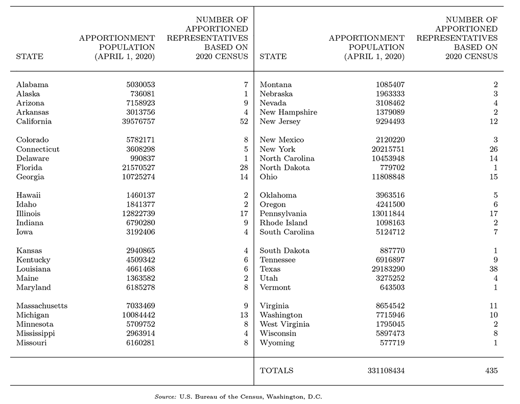
On April 26, 2021, the US Census Bureau passed to the US Commerce Department, which then delivered to the president, the 2020 Census count of population and new allocation of the 435 US House of Representatives seats among the 50 states, as shown in Table A. As important as this allocation of seats is following each census every 10 years, surprisingly few know the details for computing it. That is, how do we determine the number of seats each state gets based on its population? Basic arithmetic skill (multiplication, division, and taking square roots) is all one needs to remove any mystery concerning the details of the computations and to state a key property of the methodology.

Table A—2020 Census Apportionment Population and Number of Representatives by State

Article 1, Section 2, Clause 3 of the United States Constitution states:

We see early in the US Constitution that our government is a representative democracy, most strongly reflected in the US House of Representatives (hereafter referred to as the House). Each state is to be represented by a number of representatives according to its number (i.e., its population). One way to understand the phrase “according to its number” is to say that if a state’s population is 10 percent of the population of the United States, that state should have 10 percent of the representatives in the House. The process for determining the number of representatives (or seats) each state will have in the House is called apportionment. Among many topics in the constitutional excerpt, we see the first House had a total of 65 (= 3+8+1+5+6+4+8+1+6+10+5+5+3) seats and the apportionment (or allocation of these 65 seats) is explicitly given in the Constitution. This was based on population counts available in 1787. Going forward, starting in three years (1790), a census would be conducted for the entire United States, and the apportionment would be based on the counts from this census; thereafter, a census would be conducted each and every 10 years.

Method of Equal Proportions

Following the first presidential veto by George Washington (of an apportionment plan supported by Alexander Hamilton), Thomas Jefferson argued successfully for the method used to apportion the seats in the House based on the 1790 Census. While various methods have been used to apportion the seats in the House over the decades, the current method of apportionment is called “Equal Proportions,” and it was signed into law by President Franklin Roosevelt on November 15, 1941. H.R. 2665 (Public Law 291) – Apportionment of Representatives in Congress reads:

The method of equal proportions was used following the 1940 Census to apportion the now 435 seats in the House among the states, and it has been used every decade since.

Computations for Method of Equal Proportions

For method of equal proportions detailed computations, we begin to construct a table as illustrated in Table B (abbreviated). First, order the states from largest to smallest using their apportionment populations, as shown in Table A. We see California, Texas, Florida, New York, Pennsylvania, Illinois, Ohio, Georgia … and place them ordered along with their populations in columns one and two, as shown in Table B (abbreviated).

Next and along the top row of Table B (abbreviated), place the list of numbers It is important to point out that these numbers decrease as we go from left to right.

Next, we produce what are called priority values by first multiplying the population of California 39,576,757 by the number , obtaining 27,984,993, and we place it in Table B (abbreviated) as shown. Multiplying the population of California by the number , we obtain 16,157,143 and place it as shown. We continue similarly along the row for California obtaining additional priority values 11,424,826; 8,849,632; …

Next, on the row for Texas, we multiply the population of Texas by the number , obtaining 20,635,702 and place it in Table B (abbreviated) as shown. We continue as we did with California, obtaining the additional priority values 11,914,028; 8,424,490; 6,525,582; … and placing them in Table B (abbreviated). We do the same for Florida, New York, Pennsylvania, Illinois, …

When we finish computing the priority values for all 50 states, we have the full version of Table B, which includes 50 rows (one for each state) and 54 columns of priority values.

To determine an upper bound on the number of columns to use, we take the ratio of the population of the largest state (California) to the national population and multiply it by the 435 seats, × 435 = 51.99471692, then round up to 52. To 52, we add at least one more column. Here, we have added two to keep column spacing consistent in the table, giving 54 columns.

The full version of Table B has so many columns that we present it in four parts. To view as one table, place the parts in order side-by-side.

Table B—(Abbreviated) Computations for Equal Proportions Method Using 2020 Census Population Counts

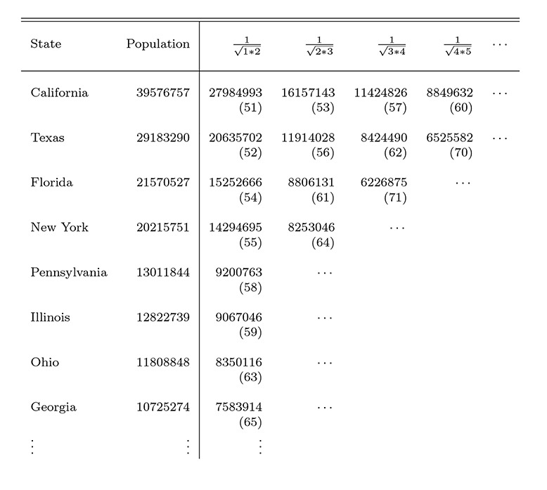
Recalling that each state gets at least one seat, the apportionment computation determines how many of the remaining 385 (= 435 – 50) seats will be allocated to each state. To do so according to the method of equal proportions, we look for the largest 385 priority values in the full version of Table B (with 50 rows and 54 columns). Because of the way we ordered the states and the numbers across the top row of the full Table B, we have a clear and interesting path for identifying these 385 largest priority values.

The largest priority value is 27,984,993, and it is associated with California, so California gets the (51st) seat. The next-largest priority value is 20,635,702, and it is associated with Texas; Texas gets the (52nd) seat. The next-largest priority value is 16,157,143, which is associated with California; California gets the (53rd) seat. The next-largest priority value is 15,252,666, which is associated with Florida; Florida gets the (54th) seat.

We continue in this fashion through the full Table B until the (435th) seat has been associated with a state. The full details are displayed in the full Table B. Careful inspection shows Minnesota gets the (435th) seat.

Finally, and for each state, we add 1 to the number of associated seats in the full Table B to get the number of seats, or representatives, based on the 2020 Census. For example, and by looking at Part I of the full Table B, we see Alabama has the associated six seats (106), (171), (231), (299), (362), and (429). Thus, Alabama gets 1 + 6 = 7 seats, as we show in Table A. The details are shown on the Alabama row of the full Table B, with its number of seats shown in the last column of the fourth part of the full Table B.

This completes a detailed illustration of how the method of equal proportions works. If there were a 436th seat in the House, which state would have gotten it in 2020? The 437th seat?

The Meaning of the Method of Equal Proportions

Ideally, we want each representative to represent the same number of people. This motivating desire is an underlying fundamental principle for the method of equal proportions.

For each possible pair of states X and Y, the method of equal proportions guarantees the number of people per representative in state X is as close to the number of people per representative in state Y as possible in a relative sense. Further, this relative closeness between a pair of states cannot be made smaller by transferring one seat for a representative from one state and giving it to the other state. This is guaranteed for all possible pairs of states.

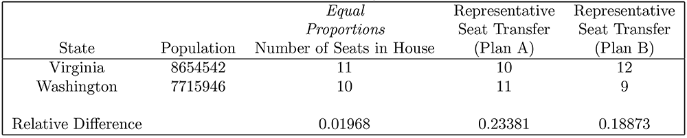
That is, by the method of equal proportions and using counts from the 2020 Census (Table A), the number of people per representative for Virginia is 8654542/11 = 786776.5455, and the number of people per representative for Washington is 7715946/10 = 771594.6000. The difference between these two numbers is 786776.5455 – 771594.6000 = 15181.9455. The method of equal proportions minimizes this difference relative to the smaller of the two numbers of people per representative. This relative difference is 15181.9455/771594.6000 = 0.01968, which is a measure of how close the number of people per representative is between these two states. This is summarized in the third column of Table C.

Can we make the people per representative between these two states closer by transferring one seat for a representative from one state to the other? There are two plans to consider. First, and for Plan A where we transfer one representative (or seat) from Virginia to Washington, the number of people per representative for Virginia is 8654542/10 = 865454.2000, and the number of people per representative for Washington is 7715946/11 = 701449.6364. The difference between these numbers is 865454.2000 – 701449.6364 = 164004.5636 and the relative difference is 164004.5636/701449.6364 = 0.23381.

This transfer has not made the two new numbers of people per representative closer in a relative sense. It has, in fact, made them farther apart. This is all summarized in the fourth column of Table C.

Second, and for Plan B where one seat for a representative is transferred from Washington to Virginia, we can proceed as in the first case, obtaining the results given in the last column of Table C, where we see the relative difference is 0.18873—again a larger relative difference than given by the method of equal proportions.

Table C—Method of Equal Proportions

Finally, one might wonder about the effect on relative difference if a seat is shifted from Virginia to Massachusetts. Would such a shift create a smaller relative difference between Virginia and Washington? The answer is no (relative difference = 0.12164).

Editor’s Note: The views presented here are those of the author and not necessarily of the US Census Bureau.